
Curation In-Depth
The Math and the In-Depth Explained.
During the last couple of weeks, Curation has captured the attention of numerous participants in The Graph’s Ecosystem. In this article, we will take a closer look at what Curation is and what the math behind it is.
Introduction.
New Discord and Telegram channels were created to facilitate communications between Curators. Those channels are proving to be an important part of our community. We highly recommend new Curators to join them.
A lot has been already achieved by these groups, but as of today there are still a lot of questions concerning the math and the in-depth concepts behind Curation. To help support the new emerging role in the ecosystem, I’ve decided to write this article to help explain the math, game theory, and economics of Curation.
First, let us zoom out and start with a general question:
This additional constraint changes the entire game. It introduces technical, game theoretical, and economic challenges.
Subgraphs on The Graph.
To make decentralized indexing possible, The Graph introduced Subgraphs. Now, Let’s zoom in on subgraphs and explore.
The Graph is a permissionless and decentralized network. Anyone or anything could publish a subgraph. This increases the decentralization of the network but introduces a new risk; fraudulent subgraphs.
If subgraphs provide API services (the core objective of The Graph), how would we ensure that indexers would index one subgraph vs another? In other words, how would the network and indexers separate good subgraphs from bad ones? What does it even mean to be a good or a bad subgraph? Luckily, we are in a digital world. Once we have determined what makes a subgraph good or bad in our opinion, we can code it and make it so.
A good subgraph is one that serves the purpose of its creation; to serve data. If a subgraph receives more queries, then it should be deemed more important than others, receiving special attention. But what type of attention? An indexer’s attention; yes, if a subgraph is deemed valuable for Web 3 it should be indexed by indexers to start collecting and organizing the data.
If a subgraph is newly deployed and still has no queries on it, how would indexers know its importance and why would they start indexing it? In other words, how does the protocol bootstrap a subgraph?
The Curation Process.
This is where Curation comes in, to bootstrap subgraphs. When Curators signal GRT on a subgraph, the subgraph becomes profitable to index. The higher the signal is, the higher the indexing rewards. Curation attracts indexing.
But what attracts Curators?
Early Curators are incentivized on The Graph. If early Curators aren’t incentivized, who will take the first step and signal on a new subgraph?
Curators could simply wait until the subgraph has proven to generate query fees, then signal.
Curator’s rewards types:

What is a Curator?
Curators explained
What are Curators and what’s their incentive? Find out!
Risks of being a Curator
Are there risks involved with being a Curator? Learn more.
We assume a Curator is a rational human being who has analyzed a subgraph and knows that a subgraph will generate query fees. Only then the Curator signals on this subgraph. If a subgraph seems not to be generating query fees, we assume that curators will move the signal onto another more valuable subgraph.
Let’s explore how curation actually works:
Bonding curves allows for the minting of new shares and burning of the old ones. If more cuators want to buy shares, the price should increase. The opposite is true as well.
This aligns with the previous point of early curators being rewarded more to help bootstrap new subgraphs. The first Curator has the least risk and maximum possible profits from selling shares, and the last Curator has the maximum risk and least possible profit from selling shares.
Let’s explain what Bonding Curves are, mathematically.
Bonding Curves.
As an example, we will consider f(x) = x2 as our bonding curve function, with f(x) := Price and x := Shares. Having Price = Shares2
Price is dominated in GRT and Shares is simply the number of minted shares on a certain subgraph.
Let’s suppose that there’s currently 1 Share minted, the Price would be Price = 12 = 1GRT.
Plotting the bonding curve:
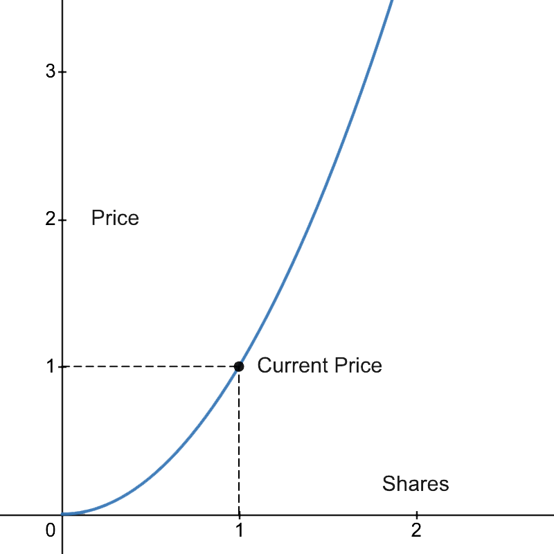
As you could see there’s 1 Share and the Current Price is 1GRT.
Looking at the figure we could see how an increase in the number of Shares will increase the Price. If someone minted an additional Share having in total 2 Shares, the Price would be Price = 22 = 4GRT
Now someone could ask: “How many GRT did we have to deposit into the bonding curve to mint 1 Share?”
We call Reserves the total amount of GRT deposited into the Bonding Curve. To calculate Reserves, we need to integrate the function, equivalent to finding the area underneath the curve as shown in the next graph.
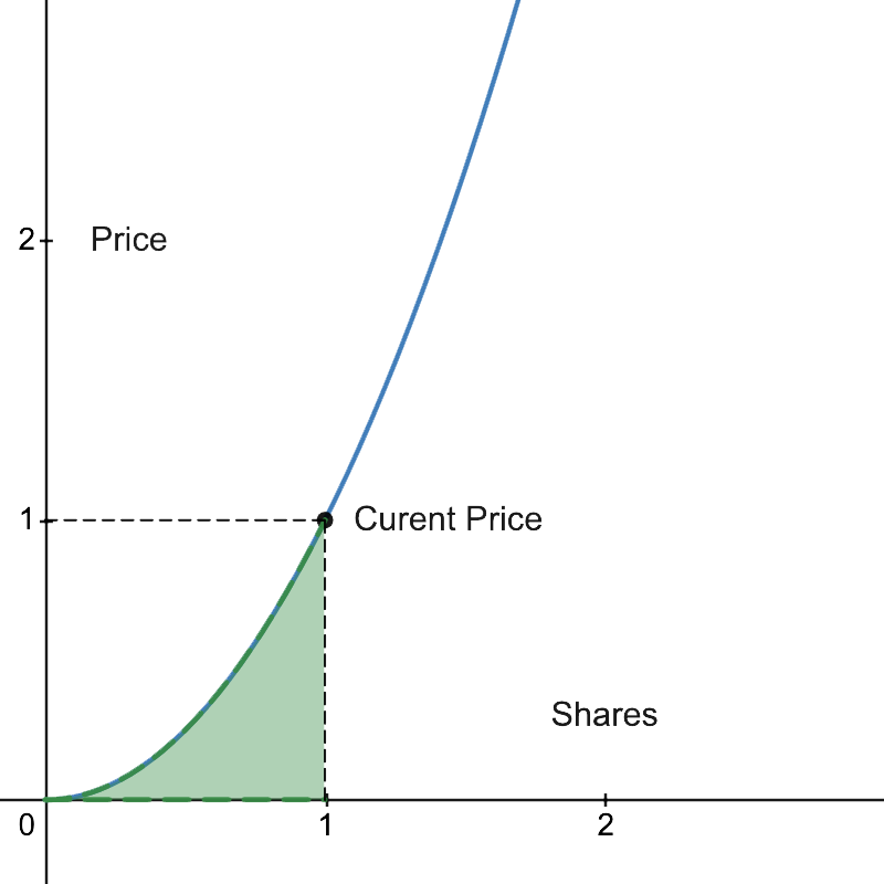
The green area corresponds to Reserves.
Reserves.
The indefinite integral would be:

The definite integral between 2 different Shares value, say a and b is:


a:=initial amount of Shares, and b:=final amount of Shares.
In our example, we were finding the Reserves between 0 Share and 1 Share, meaning a = 0 and b = 1:

It means that we had to signal 1/3 GRT to get 1 Share.
Now the following question could be:
Someone could make the mistake and say that the Current Price is 1 GRT per Share, so we should deposit 0.5 GRT to get the 0.5 Shares. Don’t forget that as Shares are minted continuously the Price changes. To solve the question is to calculate the additional amount of Reserves to be deposited when Shares increases from 1 to 1.5.
As shown in this figure:
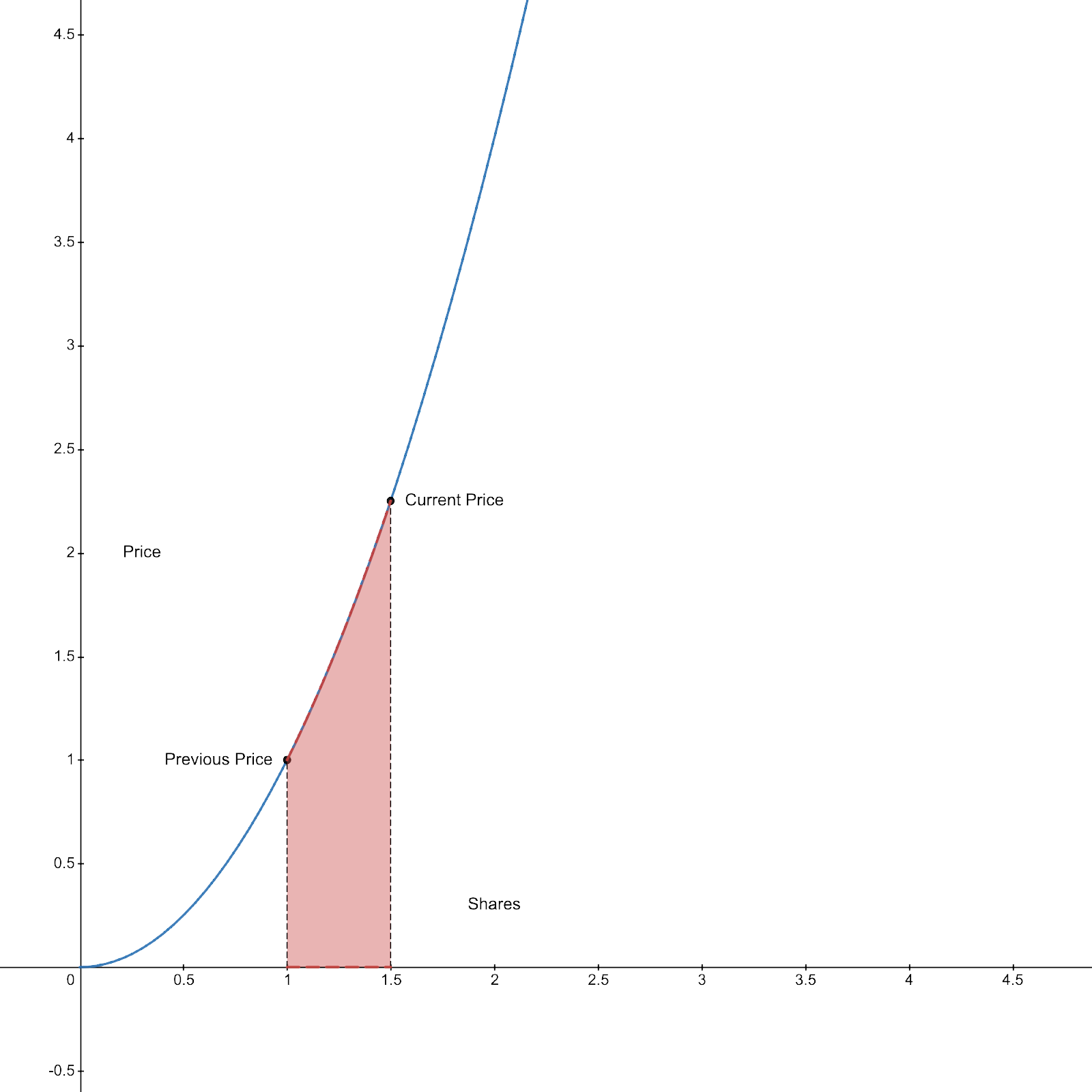
The red area is the additional Reserves to be deposited.
Using again our formula:

We replace a by 1 and b by 1.5 to find that we should deposit 0.7916 GRT.
Someone could also ask the question: “How many Shares will I get if I deposited 2 GRT?”
Let’s go back to our previous example where we had 1 Share at a Price of 1 GRT, and we knew that Reserves = 1/3 GRT.
The unknown variable in this case is b, using the same formula as before

we compute b.
Reserves = 1/3 + 2 and a = 0.
b3 = 2.333 ⇒ b ≈ 1.326
Understanding Bonding Curves will allow us to understand The Bancor Formula, which is used by The Graph protocol.
Bancor Formula.
The Bancor Formula allows the bonding curve to be defined by the Reserve Ratio.

Using the indefinite integral version we found:
and

We find:

Instead of defining our Bonding Curve by Price = Shares2, we could define it as a Bonding Curve with a Reserve Ratio of 1/3.
The reason why we would use the Reserve Ratio instead of a direct function between Price and Shares, is that at some point we would like to change the function, having a dynamic Bonding Curve, while keeping certain metrics under control.
Curators collect 10% of query fees on the subgraph. This 10% gets deposited in the bonding curve, increasing the Reserves. But as we explained before an increase in Reserves will increase Shares. But sicne no one curated more GRT, Shares shouldn’t increase. That’s why we need the ability to increase the Reserves and Price without increasing Shares. The only way to do it is to change the formula; the bonding curve itself.
Hence why The Graph uses the Bancor Formula with a dynamic bonding curve.
Here’s a graphical example:
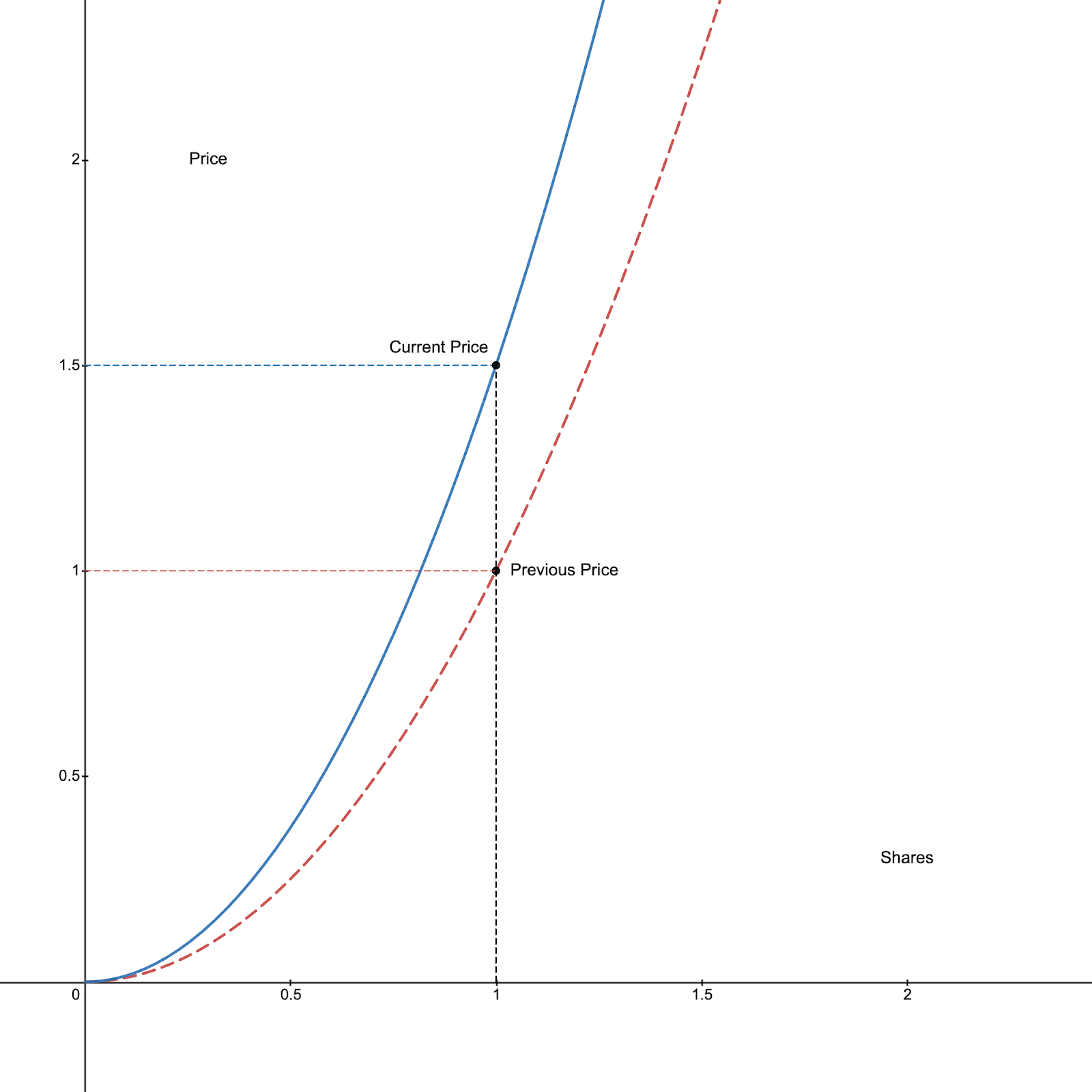
The red curve is the initial curve before depositing the query fees, and the blue one is the new adjustment that the curve had to do in order to keep the same amount of Shares which is 1, while increasing the Reserves, resulting in an increase of Price from 1 to 1.5 GRT.
We did it by changing the formula from Price = Shares2 to Price = 1.5Shares2
To understand how the formula changes, we will use the general form of bonding curves: y = mxn, with y:= Price and x := Shares

Using Bancor’s Formula:

We find:

Let’s call Reserves:=r and ReserveRatio:=Rr


That way we defined the slope m by Reserves r and the exponent n by the RerserveRatio Rr
To understand how the Bonding Curve could be dynamic, let’s say that The Graph protocol chose a certain fixed Reserve Ratio meaning n is fixed.
We said that the Price increased but the number of Shares remained the same, looking at y=mxn, we know that xn is fixed, so an increases in the price y should be the effect of an increase of m, and as we found:
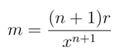
We now know that if we increase the Reserves r, m will increase, which will increase the Price.
Understanding Bonding Curves and Bancor’s Formula gives the ability to Curators to make good economic decisions. Let’s explore the economic side:
Costs.
Curators pay 2.5% on signalling as a tax everytime they signal.
Curators also have to pay an approval ETH transaction which could cost something around $2 to $3. During the time I wrote this article, the signal transaction cost around $25. ETH transactions are required as well for un-signalling. As of writing this this article, it costs around $50 to signal and un-signal, without considering the 2.5% curation tax.
Query Fees Expected Rewards.
To estimate the query fees rewards, Curators need first to pick a random Curator on the subgraph they’d wish to signal on, and look at the Curator’s proportion of shares and estimated query fees rewards. This will give a rough estimation of query fees per proportion of shares. Then, Curators need to estimate the number of shares they will mint, divide it by the total number of shares (including the estimated minted shares), to get their proportion of shares, which they’ll use to estimate the query fees rewards.
Luckily, the Graph Explorer gives an estimate of the number of shares to be minted by depositing X GRT, giving Curators all the data they need to estimate the query fees rewards.
In case of a new subgraph, where there is still no query fees, Curators can’t use the Graph Network to estimate their query fees rewards. They should do some research on the subgraph to understand its utility and usage outside of the Graph Network.
With time, Curators could derive correlations between new subgraphs and old ones, which could be used to estimate the query fees.
If you’re curious and want to derive an estimation of the bonding curve, consider the general form y = mxn, pick 2 different subgraphs with different Price/Shares that have 0 query fees deposited into their bonding curve, because query fees deposited in Reserves changes the slope m as explained before, and try to estimate m and n. You can use the following system of equations:
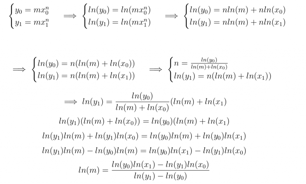

Once we have found m, we could derive n.
If you try it out on two 0 query fees subgraphs, you’ll find m=2 and n=1.
Meaning The Graph has a ReserveRatio=1/2 and an initial Bonding Curve of y=2x
The next thing is to test a subgraph that has query fees deposited in the bonding curve. Left for the reader.
Here’s some simple taste of Curation statistics:
Max Profit = 307,341.53 GRT, Max Loss = −255, 943.88 GRT, Max Return= x21.88 , Min Return= x0.04
And the graph looked like that:
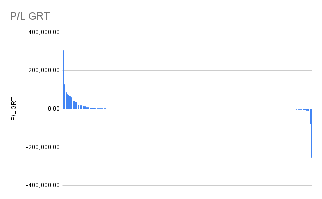
That’s a strange graph, but it sums up everything about curation for now.
Sources: “Bonding Curves In Depth: Intuition & Parametrization” by Slava Balasanov


